In our previous post we discussed how to interpret the Scores and Loadings Plots produced by PCA. In many cases there are several dimensions that are found to have substantial influence over a specific principal component, and these dimensions are often correlated in their abundance in the sample population data.

To help make sense of the results when large numbers of these variables are found, MarkerView software includes a utility to group these dimensions into a smaller number of related groups that can be more readily visualized and understood. Principal component variable grouping (PCVG)¹ is an intuitive, unsupervised data analysis method that assigns a large number of variables to a smaller number of groups that can be easily visualized. This simplifies interpretation because there are usually far fewer groups than dimensions, and the behavior of any one variable represents the rest of the group.

Members of the same group contain variables that have similar expression profiles across all samples, and some will arise from the same compound. For LC-MS, data retention time provides a further clue towards compound identification, since chemically-related ions (e.g. isotopes, adducts, etc.) will have the same retention time and can be used to indicate the molecular ion. Group members with the same retention time that are not related in these known ways can be fragments that can be used to aid structure identification. Group members that have different retention times arise from different compounds with similar behavior and depending on the experiment it might be possible to interpret these further. For instance, groups of correlated dimensions (i.e. variables that show similar response profiles across all samples) can be related biologically (e.g. co-regulated genes, biomarkers, or biochemical pathways).

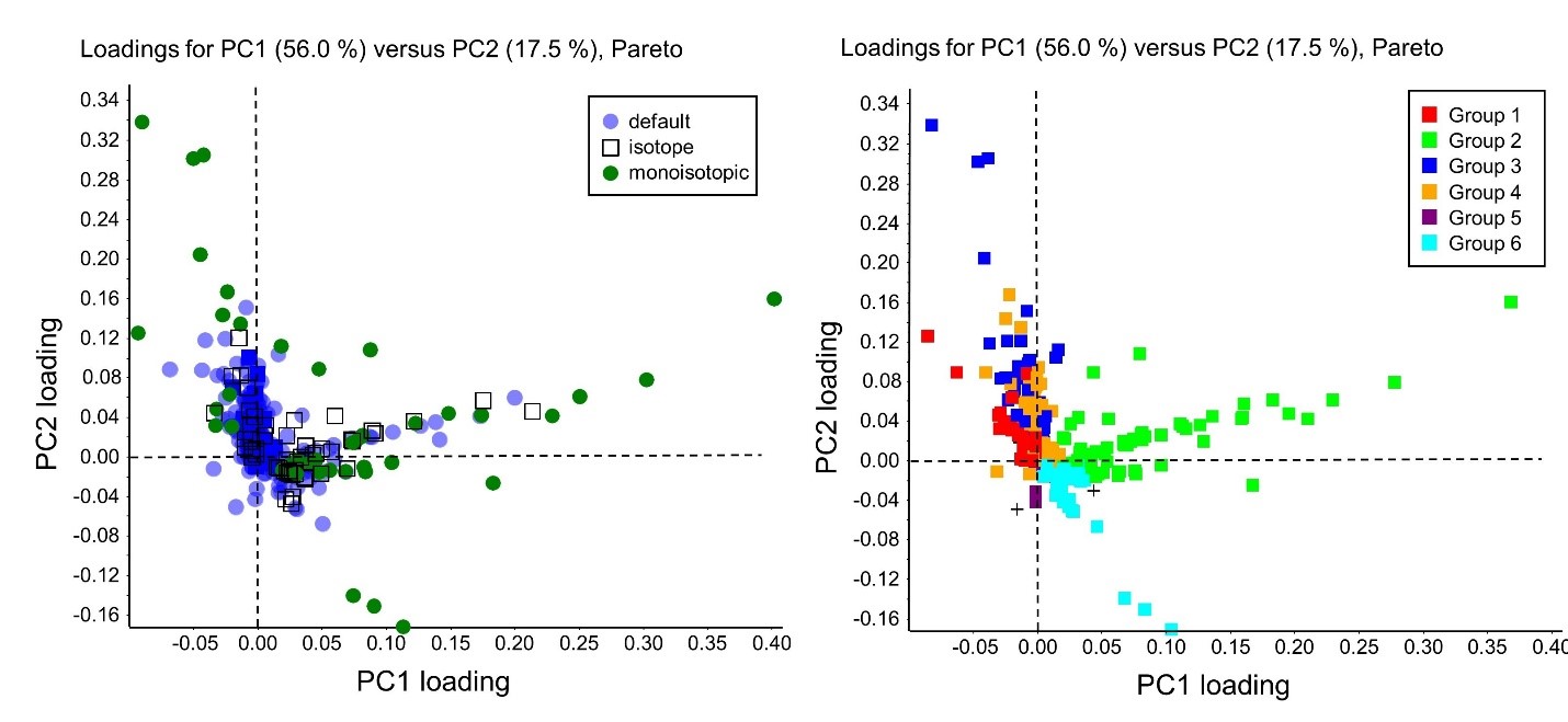
We know that the Loadings plot graphs the coefficients of each variable for PC1 versus the coefficients for PC2, and that we can use the Loadings plot to identify which dimensions have the largest effect on each component. When we apply PCVG to this example we can see several groups of correlated variables, each represented by a unique color and/or symbol in the new Loadings plot.

One way to understand how PCVG works is to imagine the Loadings plot as a three dimensional plot of all the variables exploding out from the center point.  PCVG starts at the farther point out and then “draws a cylinder” back to the center point and variables that fall within that cylinder have similar behaviors and from one group.  Then it moves on to the next farthest variable and repeats the process.

The PCVG can be run by selecting the utility Analyze > Assign PCVG Groups. This automatic version of the algorithm can be run without parameters and used to get started.

A more advanced version of the algorithm can also be used by selecting the PC Variable Grouping.exe application from the Help > Utilities menu in MarkerView software. To use this utility you must first perform PCA using Pareto scaling, and have an active plot open in MarkerView software.

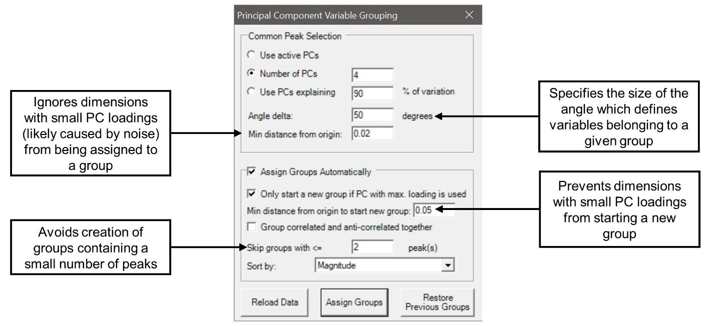
The two main parameters are the number of PCs to use, and the angle delta. To determine the number of PCs to use, remember that PCs are calculated in order of the amount of variance they describe. So, usually the first few PCs contain the important information, and the rest are mainly noise. PCVG works best using a smaller number of PCs, and this also makes visualization easier.

The angle delta, α, specifies the size of the angle that defines variables as belonging to one group or another. Note that small values can split what is probably a single group into multiple groups, and make interpretation more difficult. The number of PCs and the angle delta will depend on your unique dataset, and might require some experimentation to yield the best results. For a detailed description of the technique used to group the variables, see the references at the end of this post.

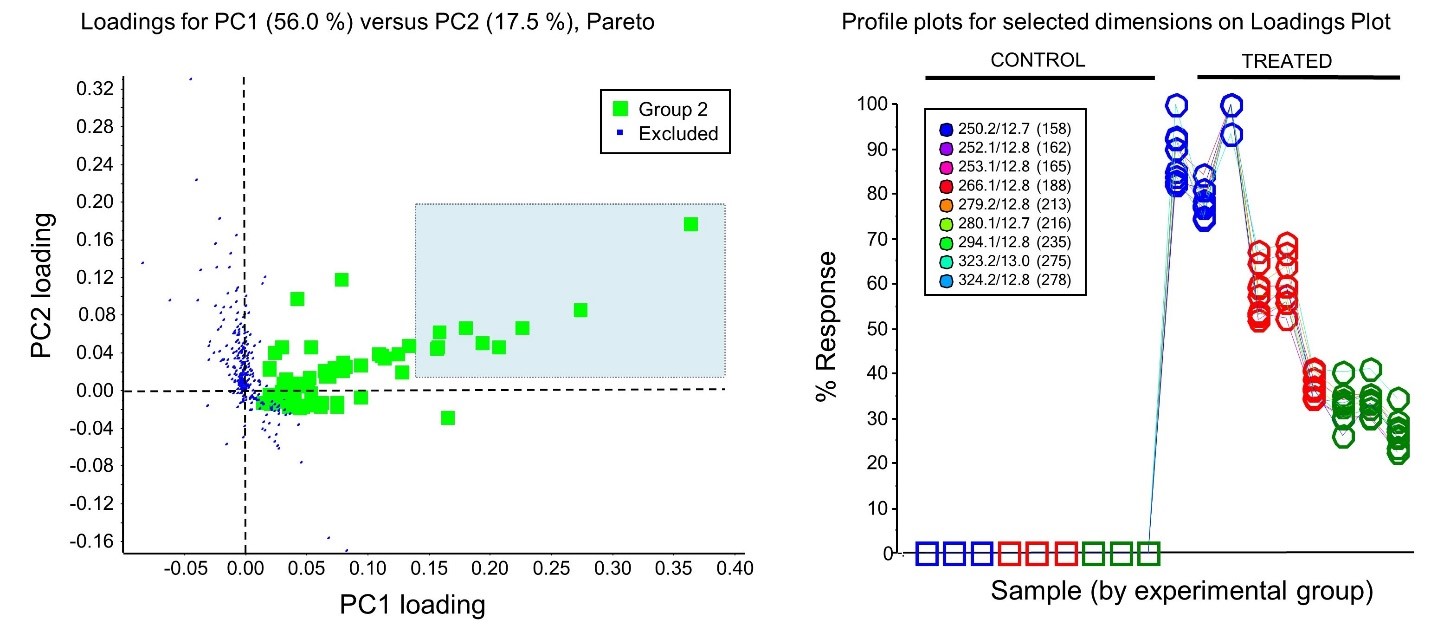
From the example above we can see six PCVG groups for further investigation. Let’s focus on Group 2 (shown in lime green). If we select the dimensions with the largest loading values (show in the blue box below), we can plot profiles for each of the selected peaks. Here we see a clear difference between the experimental groups (treated versus control). For more information about extracting information from PCA, refer to this post on T-tests.

Helpful references:

1. Ivosev G, Burton L, Bonner R (2008) Dimensionality Reduction and Visualization in Principal Component Analysis. Chem., 80 (13), pp 4933-4944.
2. MarkerView software reference guide – C:\Program Files (x86)\SCIEX\MarkerView 1.3\Help

RUO-MKT-18-12137-A